By: Armand Emamdjomeh, Washington Post interactive graphics reporter

Armand Emamdjomeh is a graphics reporter at the Washington Post who specializes in interactive maps and graphics. Aside from making maps, he enjoys running and biking and making perfectly acceptable tacos in D.C. Before coming to the Post, he worked on the graphics and data desks at the Los Angeles Times.

To say that elections are a big story in Washington, D.C. would be quite the understatement. They are the big story. For a town built around government and politics, it’s the Super Bowl, Oscars, and Kentucky Derby all rolled into one.

There are many, many approaches to creating classically-designed election maps. You’ve seen them; they’re everywhere on election night. They’re displayed on a blank background, showing the continental U.S. typically with Alaska and Hawaii positioned underneath. They’re designed to give you a quick overview of what’s happening as the results come in.

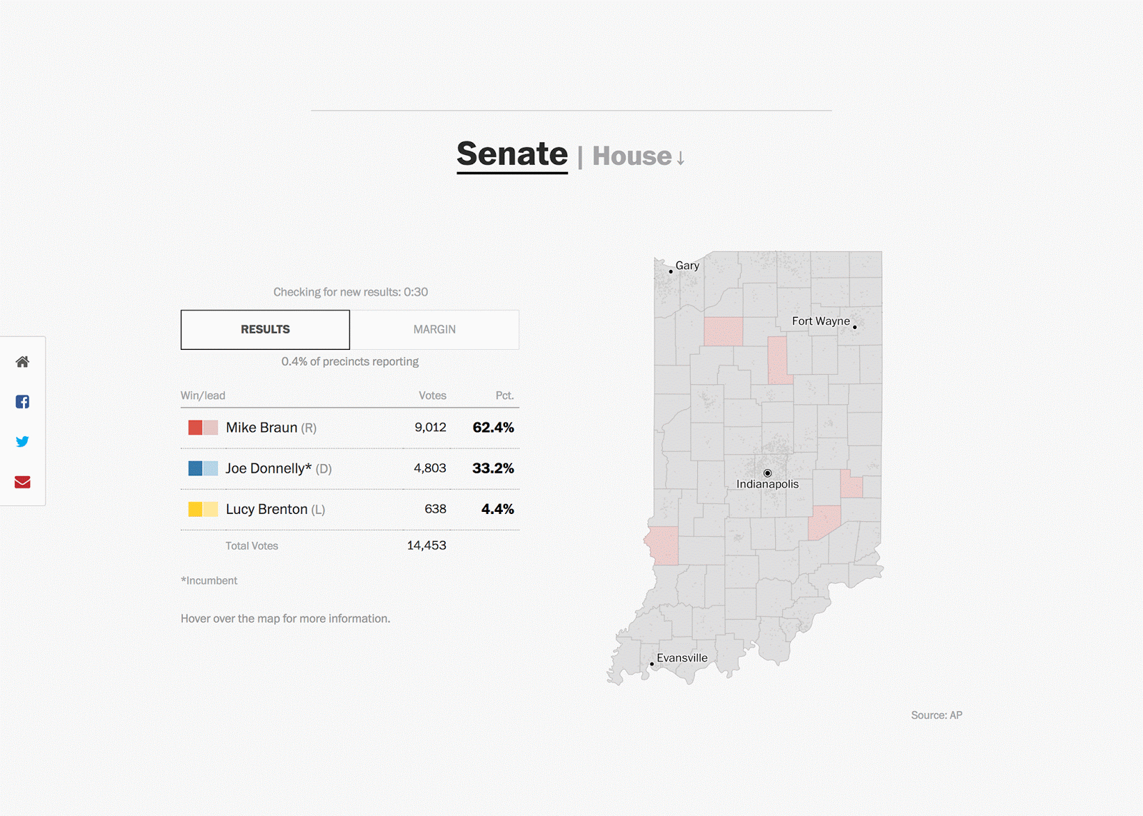
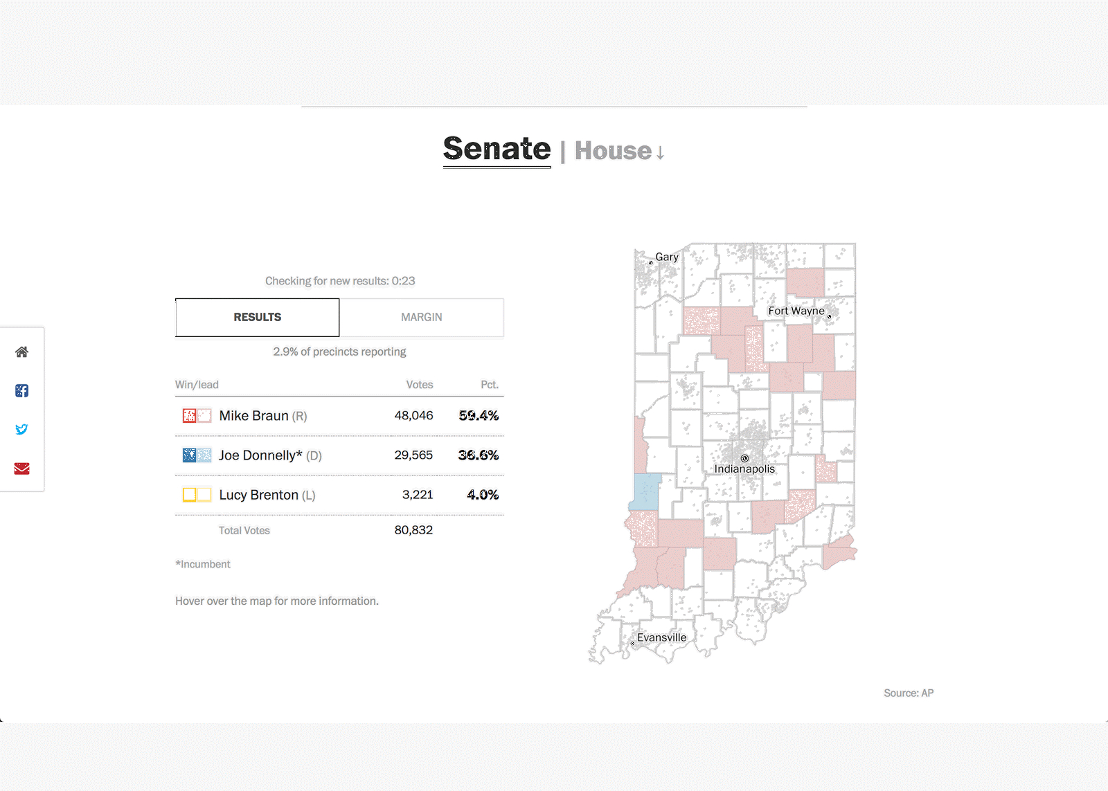
At the Washington Post, we wanted to display the election maps everyone is familiar with, but we also wanted to provide a fast interactive experience. That’s why we chose to build our election maps with Mapbox. Using a vector mapping service means we can scale the detail of our maps to fit the zoom, and mix and match custom data layers to display different forms of elections results. Also, using the new Feature State API meant we could push data updates to our features more quickly, and that interaction with the maps themselves would be faster

We originally built our election map app in 2016, and since two years is an eternity in the world of online media, there was a lot that we needed to rebuild or refactor, including how we integrated Mapbox itself. This new update not only helped us in publishing performant interactive maps on a desktop, but it also enabled us to make those interactive maps available on mobile as well, which is a huge improvement from our 2016 election rig. Here is a look at how we upgraded and built our 2018 midterm election maps.

Live data update with Feature State and Expressions

Feature State

Election maps have to be fast, legible, and easy to understand. This is where feature-state and expressions for data-driven styling come into play.

The first thing we had to address was how the map managed and updated election data. Previously, we did this using custom-built data types that modified the properties of the map features and required us to use a forked and heavily modified version of the library that kept us from keeping up with the latest updates in the Mapbox GL JS library.

Luckily for us, the new Feature State API was just released into beta and has been a part of the library now since v0.46.

Feature state allows us to dynamically set and update properties on a feature in a source. So as vote totals update in real time and races are called for one candidate or another, we can quickly update the visualization to show the latest results.

When ingesting election results, our app takes the data for each reporting unit (counties, congressional district, etc.), and makes sure any corresponding features are updated in the app. So if d here is the data for the reporting unit:

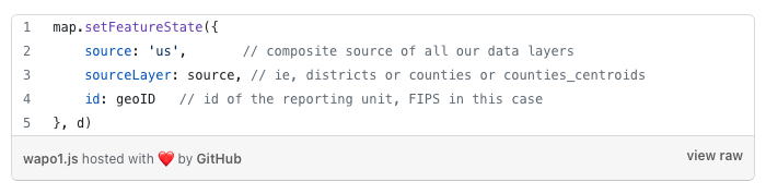
The advantage of using feature-state is that since we’re updating on a feature in a layer source rather than on a specific layer, the updates automatically carry through to any map layers that use that same source, keeping all of our maps in sync without any added overhead.

A couple of important caveats to updating data with feature-state:

• Your data must have a GeoJSON ID on the feature itself, not the properties.
• This ID must be an integer.
• As of right now, you can only use feature-state to update paint properties on a feature, not layout properties or filtering. This can make things like hiding a layer based on a feature-state difficult. We worked our way around this by reducing the opacity of features we wanted hidden to 0.
• Because of this, and because feature-state is built for updating dynamic data, we found it most useful to keep any data that won’t change — like state or county names and FIPS codes — in GeoJSON properties. This enables you to also use them to update layout and other options.

For more on feature-state and how to use it, check out this guide.

Expressions

Getting the data in is one thing. Now, we need to style it. Mapbox expressions are an incredibly powerful way to set dynamic style rules that respond to variables like data properties and zoom levels. While powerful, the syntax can be tricky if you’re building an expression from scratch, and we found it useful to pay close attention to indentation.

For example, to create a case expression that maps three possible outcomes of a race to a corresponding color:

Practically speaking, we had a function build this expression from all the possible race statuses and color mappings for a layer, but you get the idea.

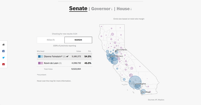
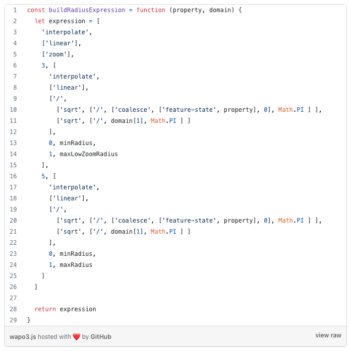
Expressions can sometimes get a little wacky. For example, the circles representing vote margins take a property and a domain corresponding to the range of margins of victory in a set of races. The radius of the circle is based on a circle with the area of the current feature-state value divided by the max, which gives us a value between zero and one, which outputs a radius between the minimum and maximum radius.

In plain English, that means larger vote margins create bigger circles.

We also wanted to interpolate the size of the circles based on the map zoom. At lower zoom levels, you want to have smaller circles, since they’re going to be more tightly spaced and more likely to overlap. As you zoom in, map features naturally grow farther apart, so we can have larger circles.

Map Projections

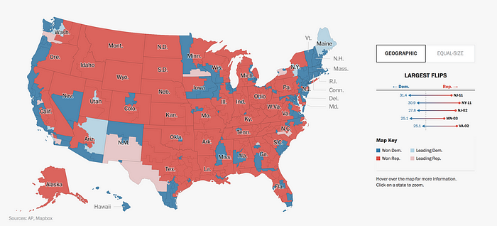
Another thing to consider when creating maps is which projection to use. At the Washington Post, our style is to show the continental United States in an Albers USA projection, a conic equal-area projection that minimizes distortion, with Alaska and Hawaii positioned under the southwestern states.

But wait, mapping services like Mapbox can only work with Mercator projection, right? Otherwise, how does it know what tiles to show?

Well, the secret part of “slippy” maps — a map that you can pan and zoom — is that they don’t care what data you’re trying to show, just that the data has consistent coordinates. So, using a technique informally called “dirty reprojection”, our maps start out with geographical data that gets projected into Albers, and then scaled to fit within a Mercator projection.

This has some weird effects — if you compare it to a standard base tile layer, the U.S. is centered over Null Island, stretching out over the Atlantic and West and Central Africa.

We generated our map data using a series of Makefiles that let us download, convert, process, and upload the data from the command line. To do this we had to:

• Download the shapefile. In our process, this is a simple Make command that uses cURL to download a zipped file from the U.S. Census.
• Extract the shapefile and perform any needed filtering (extracting U.S. states, for example.)
• Convert the shapefile to GeoJSON, and join it with data containing state names, FIPS code etc.
• Merge our three main shapes — states, counties and House districts, into one TopoJSON file with Mapshaper. Converting to TopoJSON helped to make sure we kept consistent topologies across our layers, especially as we’d be simplifying the layers to use at different zoom levels.
• Re-project the data into our pseudo-Albers projection. You could use Development Seed’s dirty-reprojectors node package for this.
• Simplify the shapes into the three main simplifications we used — high, mid and low-detail shapes. This way you’d see nice detail when you’re zoomed into a single state, but would have a lower-detail (and lighter) layer when you’re looking at the national view. Since they’re all still in one merged TopoJSON file, the shapes and boundaries are going to be consistent. We output the layers into separate GeoJSON files.
• Convert our GeoJSON into MBTiles with Tippecanoe. Since we have three separate zooms for each type of geometry, we convert each of those to its own layer, specifying which zoom levels it will be used for. And since we’re using projected coordinates, you need to tell Tippecanoe that by using — projection EPSG:3857 in your command line. We’ll join these output layers together immediately after using tile-join.

tiles/%-z4-6.mbtiles: geojson/albers/us-lowzoom/%.json
 mkdir -p $(dir $@)
 tippecanoe --projection EPSG:3857 \
  -f \
  --named-layer=$* \
  --read-parallel \
  --no-polygon-splitting \
  --detect-shared-borders \
  --minimum-zoom=4 \
  --maximum-zoom=6 \
  --drop-rate=0 \
  --name=2016-us-election-$* \
  --output $@

“Make” rules like this one are just intermediary steps and you’d never actually call that command directly. Instead, we’d call something like make tiles/election/states.mbtiles. That would trigger the entire process, downloading and processing shapefile if needed, and creating our final tile layers.

• After making the tileset, it’s important to see what you’ve created. You can use mbview to preview the MBTiles that you’ve just created. This will allow you to verify that your geometries and properties are what you expect before uploading to Mapbox.
• Now you’re ready to upload! Instead of directly uploading through the Mapbox interface, we used the Mapbox command line interface to upload our tilesets. This enables us to keep everything in the command line, but more importantly, we can specify a tileset ID, which the Mapbox studio interface doesn’t allow. Specifying a tileset ID is super helpful when keeping track of a bunch of tile layers.

Here is an example upload command to upload our House districts file with a tileset ID of washingtonpost.2018-election-districts-v1:

mapbox upload washingtonpost.2018-election-districts-v1 tiles/election/districts_2018.mbtiles

The process had a couple of extra steps depending on the data we were trying to output. For example, U.S. House districts needed to include a redistricted Pennsylvania, so we had to remove the old Pennsylvania districts, and replace them with the redistricted shapes we got from a separate source. Additionally, since the House district shapefile isn’t clipped to the U.S. shoreline, we clipped those in an another step.

To keep the appearance and relative scale of map features consistent, you want to re-project before simplifying, or the simplification will appear uneven because Alaska and Hawaii change in scale in an Albers USA projection

One caveat with this approach is that if you’re showing a single state, it can look very strange in an Albers USA projection, like the jauntily-angled Virginia map, below.

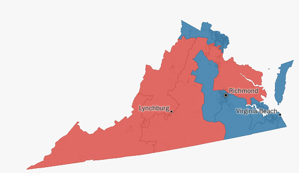
States close to the coast, for example, will appear unnecessarily rotated. So we wanted to show individual states in a standard Web Mercator projection, which meant that we had two versions of each layer, Albers and Mercator, and changed the sources as needed.

Keep in mind that when you are using these projection tricks, nothing will be where you think it will be. That means that you’ll have to figure out what the bounds of your projected shapes are if you want to zoom to a specific state or district, for example.

Election Cartogram

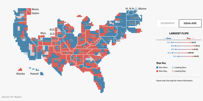
There is another style of maps that is making its way into the traditional election visualizations: the cartogram. Cartograms are maps that are distorted by a variable, by population or GDP, for example, to favor information over geography.

Before we dive into it, you must be wondering why cartograms are used so frequently in elections coverage. They look weird, they’re not geographically accurate, and people get confused by them. But, the lack of geographical accuracy is why they’re so useful in the first place. They’re one of the only ways to accommodate for the fact that population density is not the same across the country. Due to population density, urban areas can be greatly under-represented in a geographic map.

For example, the state of New Jersey has roughly the same population as the states of Idaho, Wyoming, Utah, both Dakotas and Nebraska, combined.

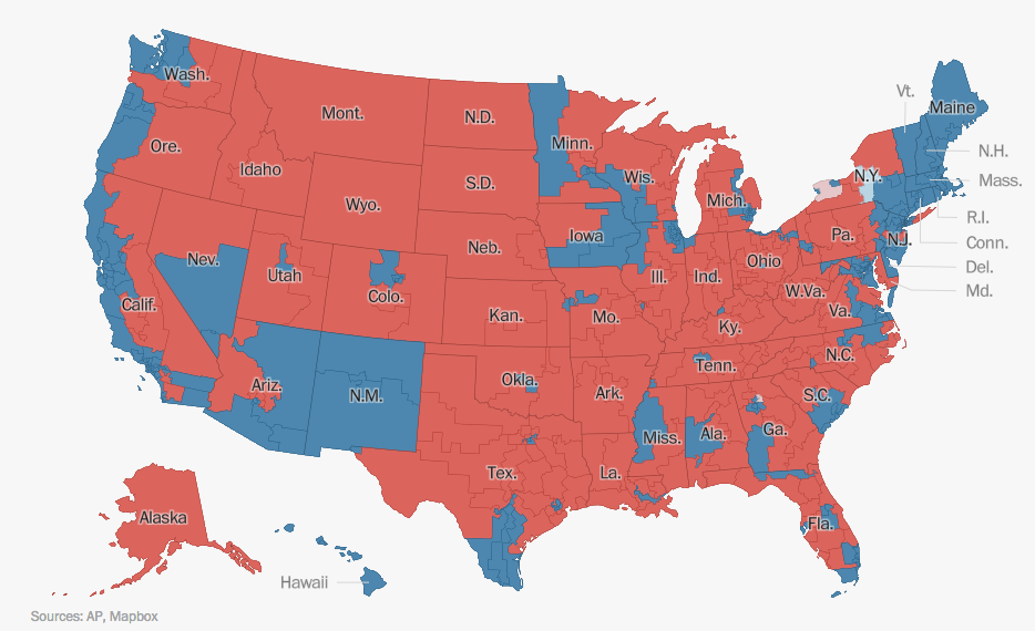
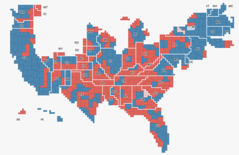
A geographic map of U.S. House results, then, appears as if there are very few Democratic representatives, when in fact they now hold the majority of seats. It’s just that most districts are too small to see at a national level. By using cartograms with equal-sized units for each legislative seat, we can try to provide a more accurate view of the proportional results.

At first glance, creating a cartogram seemed like a particularly tricky problem: how do we get a map designed in Adobe Illustrator into a Mapbox slippy map?

This is actually simpler than it seems. A map doesn’t care what coordinates you use. All it cares about is that these coordinates are consistent in relation to each other. Since SVG paths are essentially arrays of coordinates, SVG paths can simply be converted into GeoJSON features

One key element to be aware of as you convert an SVG into a GeoJSON is to have a way to identify each feature. Since we wanted to roughly locate every district in the cartogram to help better represent the political makeup of each state, we made sure that each path had an ID. So in the Illustrator file, we added a layer ID to each path, (e.g., CA-28) and preserved that in the GeoJSON feature properties. Note that in the image, CA-28 is nowhere near its geographic position in Southern California, there are just that many districts!

We wrote a custom node.js script that converted our cartogram SVG for use specifically with our app, but Mapbox also has its own svg-to-geojson script.

Custom Labels and re-projection

State and city labels were another tricky task, especially since we were using an Albers projection, and at a national level, state labels over small states will either collide, or not be displayed altogether.

How did we do it? We drew our own custom pointers.

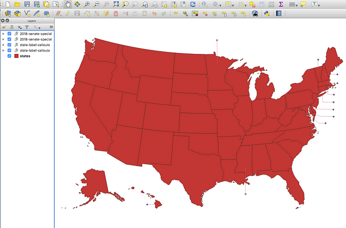
The regular state labels (the ones without the callouts) were created by getting the centroid of each state. We aggregated those into a point layer, with each point associated with the FIPS code and AP abbreviation for its state, as well as the postal code, which we used for lower zooms. We then displayed these as a symbol layer in Mapbox.

The callouts were a little more complex. These can be created by drawing your own custom shapes in QGIS. Since these lines have their own geometries you can also convert them to GeoJSON and they’ll show up, just like any other map feature! You want to make sure to draw the callouts on your Albers-projected geometry, otherwise you’ll wind up pointing to the wrong coordinates.

For more on election maps, check out our three-part series exploring feature-state, expressions, and map design. As always, if you have questions, you can email Lo at lo@mapbox.com or find them on Twitter, Lo Bénichou.

‍