With the 0.41 release of Mapbox GL JS (and mobile SDKs to follow), we’re introducing heatmaps — a beautiful way to visualize and explore massive point datasets.

A heatmap is a data visualization where a range of colors represent the density of points in a particular area. Heatmaps help us see the “shape” of the data and highlight areas of concentration where many points are clustered closely together. The dynamic heatmap layer in Mapbox GL JS renders smoothly at 60 fps while panning and zooming. It’s fast and can handle large amounts of data (especially when combined with clustering). Let’s see what an interactive heatmap of 400,000 points looks like:

Getting started with heatmaps

If you want to get started with heatmaps right away, dive into our official example or take a look at a detailed tutorial. Want to know more? Read on for an overview.

You can start by adding a layer with type 'heatmap' to your style:

Heatmaps can require a lot of customization based on your use-case. Thankfully, Mapbox GL JS provides a set of powerful paint style properties for controlling every aspect of the layer’s appearance in real time.

map.addSource('earthquakes', {
	type: 'geojson',
	data: 'earthquakes.geojson'
});
map.addLayer({
	id: 'earthquakes',
	source: 'earthquakes',
	type: 'heatmap'
});

heatmap-radius

This property affects how detailed the heatmap will be by setting the “radius of influence” of each point in pixels (an equivalent of the bandwidth parameter in kernel density estimation). Higher values make for a smoother, more generalized look. The property can also be a zoom function, allowing you to adjust the look as you zoom in.

‍

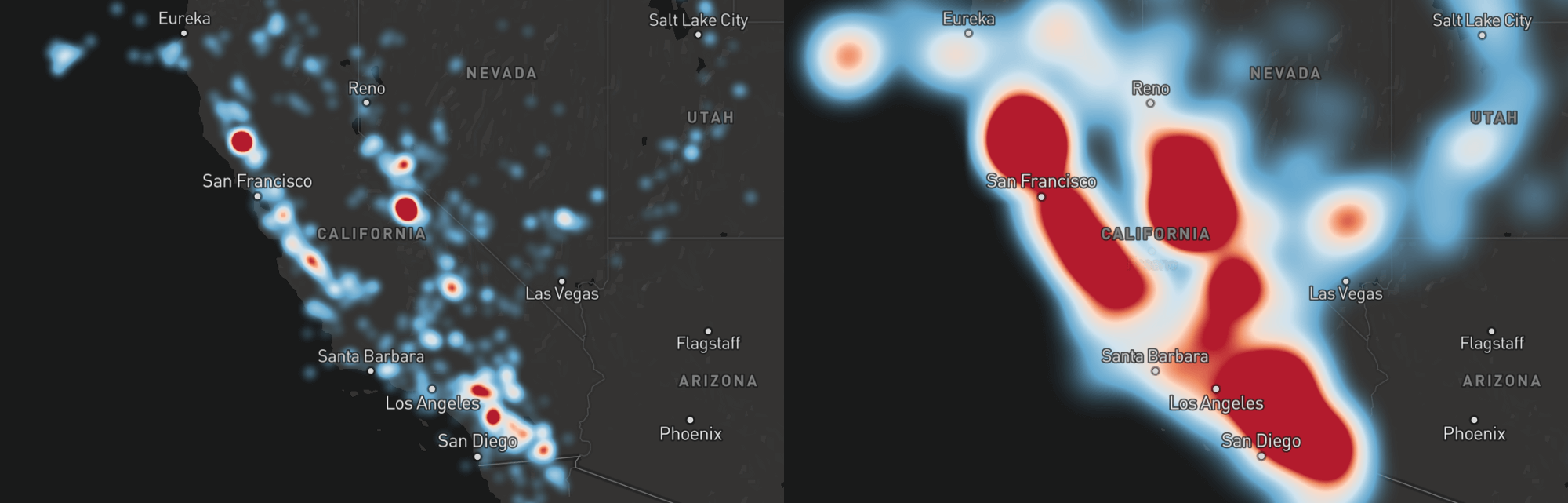
This style property controls the most important aspect of heatmap design — how the “density” value of each pixel on a map translates to color:

The value of the property is a function which maps density values ranging from 0.0 to 1.0 to colors. This example will make the most sparse areas blue while gradually transitioning through yellow to red at the most crowded spots.

"heatmap-color": {
	"stops": [
		[0.0, "blue"],
		[0.5, "yellow"],
		[1.0, "red"]
	]
}

heatmap-color

This style property controls the most important aspect of heatmap design — how the “density” value of each pixel on a map translates to color:

The value of the property is a function which maps density values ranging from 0.0 to 1.0 to colors. This example will make the most sparse areas blue while gradually transitioning through yellow to red at the most crowded spots.

"heatmap-color": {
	stops": [
		[0.0, "blue"], 
		[0.5, "yellow"], 
		[1.0, "red"]
	]
}

heatmap-intensity

This property allows you to adjust the intensity of the heatmap appearance globally. The higher the value, the more “weight” each point will contribute to the look. The relation is linear — e.g., setting heatmap-intensity to 10.0 is equivalent to duplicating the dataset ten times and rendering it with the default 1.0 value.

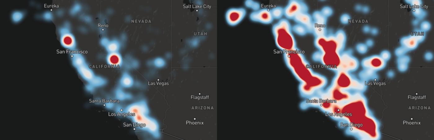
heatmap-intensity is very useful for adjusting the look of the heatmap to different zoom levels — if you leave it constant, the heatmap on lower zooms will look much heavier because points will be visually closer together.

heatmap-weight

This style property works the same as heatmap-intensity, except that it can be data-driven, adjusting intensity of individual points depending on their feature properties:

"heatmap-weight": {
	"type": "identity",
	"property": "point_count"
}

In this example, a point with point_count value of 100 will look the same as 100 points with point_count of 1. Combined with clustering, this improves heatmap performance by drastically reducing the number of points to draw.

heatmap-opacity

This property controls the global opacity of the heatmap layer.

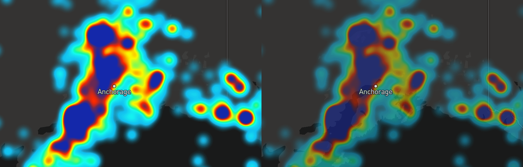
One useful application of heatmap-opacity is fading out the heatmap for a more detailed look when zooming in:

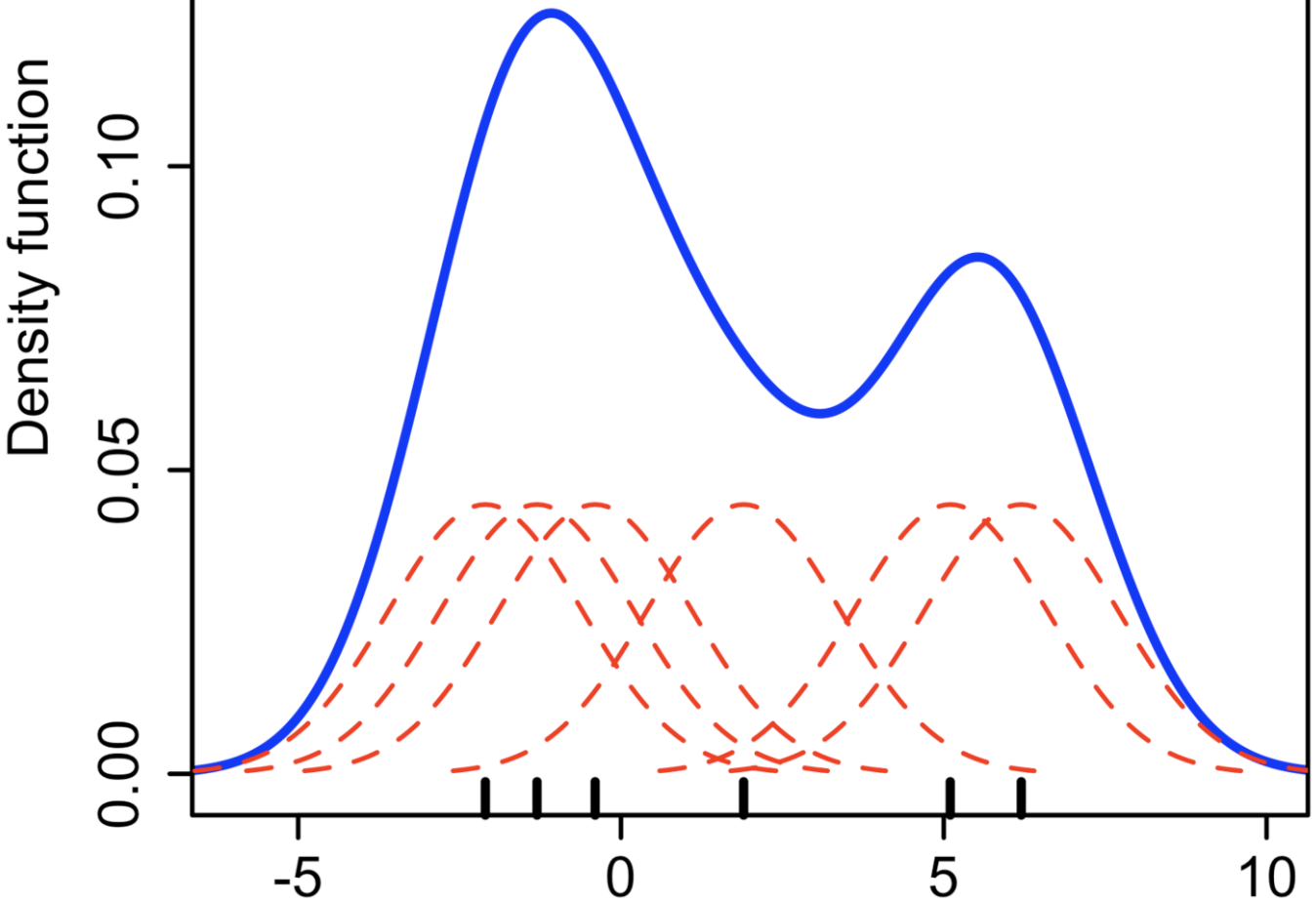
How heatmaps work under the hood

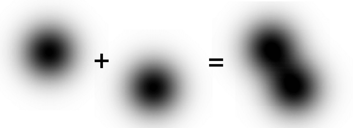
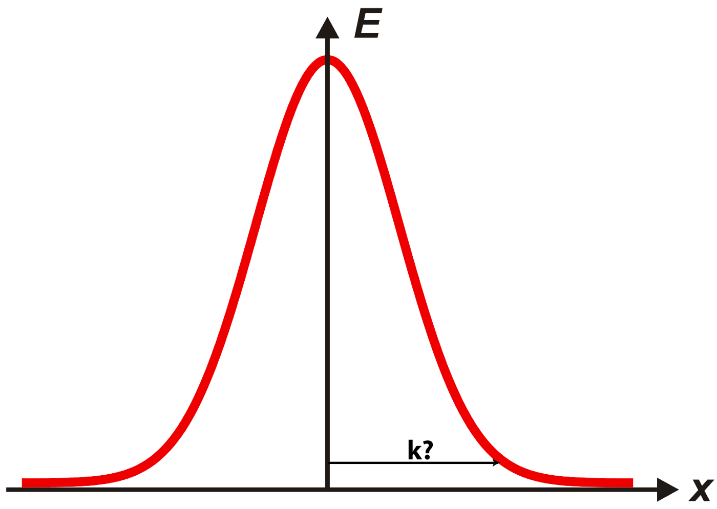
In mathematical terms, Mapbox GL heatmaps are a bivariate (2D) kernel density estimation with a Gaussian kernel. It means that each data point has an area of “influence” around it (called a kernel) where the numerical value of influence (which we call density) decreases as you go further from the point. If we sum density values of all points in every pixel of the screen, we get a combined density value which we then map to a heatmap color.

To implement this with OpenGL, for each data point, we draw the kernel (which looks like a blurred circle) into an offscreen half-float texture with additive blending (so that values are summed together when kernels overlap), and then we colorize this greyscale texture in a separate step.

Ideally, we need to calculate density for every screen pixel separately for each data point because this value never becomes fully zero, even when far away from the corresponding point. But that would be too expensive — even a modest amount of points to draw would require billions of operations. To speed things up, we crop each kernel to a square that’s just big enough for all values outside to be very small (under a certain threshold — we arbitrarily picked 1 / 255 / 16). This size will depend on weight and intensity of each point; heavier points will need a bigger drawing area.

Additionally, for drawing the densities, we use a downscaled texture with 4 times smaller sides than the map resolution (resulting in 16 times fewer pixels to draw for each point), and then upscale the texture back with linear interpolation during the colorization step. For heatmaps, this is visually almost indistinguishable from full resolution rendering, but it makes it considerably faster.

A different approach to heatmaps

Other platforms render heatmaps as static image tiles on the server. Our approach to heatmaps takes advantage of Mapbox GL at its core, rendering smooth transitions at 60fps and providing the ability to control every aspect of heatmap layers at scale — from picking the right color ramp to adjusting the point radius at each zoom level. Combine heatmaps with other GL JS capabilities like data-driven styling, expressions, and clustering for more unique configurations of your data.

Thank you for reading! Check out this example and tutorial for heatmaps in GL JS, and stay tuned for the launch of this feature in our mobile SDKs later this year. Reach out on Twitter (@mourner) or respond here in Medium if you have questions or comments. Let us know what you make with the tag #BuiltWithMapbox.

‍